Methods of Communication
Research and Statistics
Online Workbook
Selection Charts
Before you can start calculating a particular test statistic, you must first decide which measurement(s) can actually be calculated. This is because the measures that you can calculate depend on the number of variables, the levels of measurement of these variables, and the 'substance' of what you want to know (e.g. Do you want to determine an association or a difference? Should the association be symmetrical or asymmetrical?). There are several selection charts that are relevant to Methods of Communication Research and Statistics e.g. for determining the level of measurement for a variable, for generating graphs, for measures of central tendency, for measures of dispersion, and for measures of association. You can usually consult the selection charts via the hints accompanying an exercise.
Level of measurement decision diagram
| You can determine the correct level of measurement of a variable by running through this chart. Begin with the first question. | QUESTION 1: Does one value mean something different to another? E.g.: Is sitting in front of your computer for one hour slightly different to sitting there for two hours?
- If not: this variable is meaningless. - If so: go to question 2. Explanation: This is called the identity relationship. It's hard to find a variable that does not meet this requirement. |
Meaningless |
| QUESTION 2: Can you say that one value is greater or lesser than the other? E.g.: is sitting in front of your computer for two hours longer than sitting there for one hour?
- If not: this variable is measured at a nominal level of measurement. - If so: go to question 3. Explanation: If only a name is involved, or categories that are not related in terms of being 'greater' or 'lesser' than each other, we refer to this as nominal. E.g.: gender ('male' is not greater or lesser than 'female'); which newspaper someone reads ('NRC' is not greater or lesser than the 'Volkskrant'); place of residence, etc. |
Nominal | |
| QUESTION 3: Can you say how great the difference between two values is? E.g.: can you say there is a difference of one hour between sitting in front of your computer for one hour and sitting there for two hours?
- If not: this variable is measured at ordinal level of measurement. - If so: go to question 4. Explanation: If there is a specific ranking (e.g., 2 is more than 1), but you do not know anything about the difference (the intervals) between these two values, there is said to be an ordinal level of measurement. E.g.: levels of education (a Bachelor's degree is 'lower' than a Master's degree, but you cannot say exactly by how much); age categories (someone in the 30-40 age category is older than someone in the 18-25 category, but you cannot say exactly how much older). |
Ordinal | |
| QUESTION 4: Can you say that one value is worth twice as much as another? Is it impossible for negative values to occur? E.g.: can you say that sitting in front of your computer for two hours is twice as long as sitting there for one hour?
- If not: this variable is measured at an interval level of measurement. - If so: this variable is measured at a ratio level of measurement. Explanation: Variables that are measured using a fixed unit (e.g. where the answer to question 3 is 'yes') may be used in calculations. These values can be added and subtracted, multiplied and divided. If negative values are possible, there is no absolute zero. This is then an interval level of measurement. If there is an absolute zero, then this is a ratio level of measurement. |
Interval / Ratio |
Graph selection charts
| Bar chart | Pie chart | Box plot | Histogram | ||||||
| 1. Select | 1.1 Specifics | How often does something occur? | What things occur relatively often? | What is the dispersion like within a variable? | What is the shape of a distribution? | ||||
| 1.2 Minimum level of measurement | Nominal | Nominal | Ordinal | Interval | |||||
| 2. Calculate | Frequencies -> Charts -> Bar | Frequencies -> Charts -> Pie | Graphs -> Legacy dialogs -> Boxplot | Frequencies -> Charts -> Histogram | |||||
| 3. Check | The graph must have a title, names and scales on the axes and, if applicable, acknowledgement of the source. | ||||||||
| 4. Conclude | Select a few notable values and mention them, indicating what the units are and what the variable means. | Describe the centre of the distribution, the limits of the middle half of the observations, skewness, and extremes. | Describe the shape of the distribution (number of peaks, symmetry, and skewness) and several notable points (peaks, troughs), clarifying what the units are and what the variable means. | ||||||
Measures of central tendency and measures of dispersion selection chart
| Measure of central tendency | Mode | Median | Mean | |
| Measure of dispersion | Interquartile range | Standard deviation, Variance | ||
| 1. Select | 1.1 Specifics | What occurs most frequently? | What is the median value? | What is the balance point of the distribution? |
| 1.2 Minimum level of measurement | Nominal | Ordinal | Interval | |
| 1.3 Shape of the distribution | Usable with every distribution shape | Usable with every distribution shape | Not optimal for very skewed distributions | |
| 2. Calculate | Analyze-> Descriptive Statistics -> Frequencies -> Statistics | Analyze-> Descriptive Statistics -> Frequencies -> Statistics | Analyze-> Descriptive Statistics -> Frequencies -> Statistics | |
| 3. Check | Unusable with a distribution with many peaks, e.g. in the case of an ungrouped interval variable. | The greater the difference between the mode, median, and the mean, the more skewed the distribution. | ||
| 4. Conclude | General:
1. Give your reasons for selecting the measure of central tendency and measure of dispersion (see Select and Check). 2. Use the value of the measure of dispersion to comment on the accuracy of the calculated measure of central tendency: the smaller the distribution, the better the centre typifies the distribution. |
|||
| Mode: "The most common value of variable X is A.". | Median: "The median value of variable X is A" or "Half of the units of analysis have A or less on variable X, and half of the units of analysis have A or more on variable X." Interquartile range: "The mean deviation from variable X compared to the median is A" or "The middle half of the observations lies between (first quartile limit) and (third quartile limit). |
Mean: "The units have an average A on variable X." Standard deviation, Variance "The mean deviation in relation to the mean." |
||
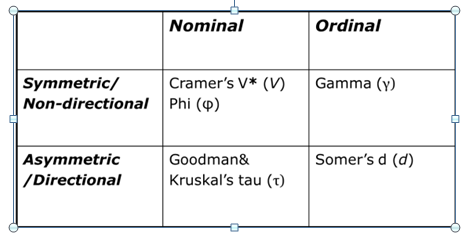
Measures of association
Irregular measure: Eta/Eta2, which is used whenever the independent variable is categorical (nominal or ordinal) and the dependent variable is numeric (interval or ratio).
Strength of association
0 - 0,10 |
very small/no association |
0,11 - 0,30 |
small association |
0,31 - 0,50 |
medium association |
0,51 - 0,80 |
large association |
0,81 - 0,99 |
very large association |
1 |
perfect association |
Please note: The direction of an association is indicated with a - (minus sign) when the association is negative. This is only possible with variables that are both measured at least at ordinal level.
Interpreting measures of association (and where to find this in SPSS)
The following applies to every interpretation:
- Name the measure of association and value (round to two decimal places).
- Name the strength and, if applicable, direction of the association.
- Repeat the variables to which the measure relates.
- Name the units of analysis.
- Draw a conclusion.
The following applies to every contingency table:
- Apart from the frequencies, the columns should also contain percentages.
- If you have an asymmetric relationship, put the independent variable in the columns.
- Discuss the percentages from at least two cells in the contingency table if there is an association.
We have set out below what must be included in the interpretation for each measure of association, including an example (in brackets). Although these examples discuss the variables 'X' and 'Y', variables must always be written out in full (e.g.: gender, number of hours watching television, frequency of WhatsApp usage, etc.).
Cramer's V / phiLambda / Goodman and Kruskall's tau
Gamma / Kendall's tau-b
Spearman's rho
Somers' d
Pearson's product moment correlation coefficient
Eta
Eta2
Simple regression analysis
Multiple regression analysis