Methods of Communication Research and Statistics

Using an experiment, a communication scientist wishes to find out whether seeing advertisements for snacks has an effect on children eating sweets while watching TV. 40 children aged 6 to 12 took part in the experiment. The experiment took place in a room set up as a living room, where each child spent half an hour watching cartoons on television, with a bowl of sweets on a table. In the case of half of the children, the cartoon was interrupted part-way through with advertisements for snacks. The children were allocated sessions with and without advertisements at random. The number of sweets eaten by each child during the half hour was counted by the researcher.

Database: SnackCommercial.sav

a. Test the hypothesis that the advertisements lead to children eating more sweets. Formulate the statistical hypotheses for this test and draw a conclusion.

Start by describing the variables: are there any impossible values in the variables 'Condition' and 'Sweets'? Sweets includes the value -3; it is impossible to eat a negative number of sweets, so this value must be designated 'missing'.

For each condition (category), there are just 20 observations (and 19 in the group with a missing value). This means that we can only carry out the t-test if the variable is distributed normally in the population. This information is not included in the exercise, so the only thing we can do is to check the distribution of the 'Sweets' variable in the sample. Is it not too skewed, does it follow the normal distribution, and are there any extremes beyond the tail-ends?

Using the EXPLORE command, you can ask for the skewness and boxplots with extremes to be shown. If you want a histogram with a normal distribution displayed, use FREQUENCIES.

Statistics

Sweets

N Valid 39

Missing 1

Mean 5,05

Std. Deviation 1,701

Skewness ,051

Std. Error of Skewness ,378

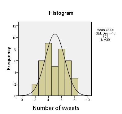
The distribution is barely skewed (skewness = 0.05) and has no extremes. The distribution in the sample is reasonably normal, although the number of children who ate five sweets is markedly lower than what would be expected with a normal distribution.

This does not provide hard evidence that the variable in the population has a normal distribution, but the reasonably normal distribution in the sample makes it fair to assume that the variable in the population is also distributed normally. We therefore use the t-test here anyway.

We have two groups (or two samples) here: the children who do, and the children who do not, see advertisements. We therefore have to carry out a t-test on two means. The null hypothesis is that there is no difference between the two means in the population. If we do not wish to rule out the possibility that children who see advertisements for snacks eat fewer sweets, we have to carry out a two-way test. The statistical hypotheses are then:

H₀: μ_{advertisement group} = μ_{no-advertisement group}
H₁: μ_{advertisement group} ≠ μ_{no-advertisement group}

Now carry out the t-test. The results are shown in the tables below.

Group Statistics

Conditie N Mean Std. Deviation Std. Error Mean

Sweets 0 no advertisements 19 3,58 ,838 ,192

1 with advertisements 20 6,45 ,945 ,211

Independent Samples Test

Levene's Test for Equality of Variances t-test for Equality of Means

95% Confidence Interval of the Difference

F Sig. t df Sig. (2-tailed) Mean Difference Std. Error Difference Lower Upper

Sweets Equal variances assumed ,441 ,511 -10,023 37 ,000 -2,871 ,286 -3,451 -2,291

Equal variances not assumed -10,054 36,834 ,000 -2,871 ,286 -3,450 -2,292

Conclusion: Children who do see advertisements eat significantly more sweets (M = 6.45, SD = 0.95) than those who see no advertisements (M = 3.58, SD = 0.84), t (37) = -10.02; p < 0.001; 95% CI [-3.45, -2.29]; d = 3.21. The effect of the advertisements is very strong. See below how this value, with the related pooled variance, is calculated by hand:

Note: We assume that eating sweets in the population has a normal distribution.
Note: Levene's test is not significant, so we may assume equal variances for the two groups in the population.

Syntax

*Describing the variables and defining missing values.
*Define Variable Properties.
*Sweets.
MISSING VALUES Sweets (-3).
EXECUTE.
*Assessing the distribution shape: normal?
*M, SD, skewness and histogram with normal distribution.
FREQUENCIES VARIABLES=Sweets
  /FORMAT=NOTABLE
  /STATISTICS=STDDEV MEAN SKEWNESS SESKEW
  /HISTOGRAM NORMAL
  /ORDER=ANALYSIS.
*Boxplot and list of extremes.
EXAMINE VARIABLES=Sweets
  /PLOT BOXPLOT
  /COMPARE GROUP
  /STATISTICS EXTREME
  /MISSING LISTWISE
  /NOTOTAL.
*t-test on two means.
T-TEST GROUPS=Condition(0 1)
  /MISSING=ANALYSIS
  /VARIABLES=Sweets
  /CRITERIA=CI(.95).

First check the 'gender' variable (no problems) and then carry out another t-test for the difference between two means.
Conclusion: Boys eat significantly more sweets while watching television (M = 5.60, SD = 1.57) than girls (M = 4.47, SD = 1.68), t (37) = -2.17; p < 0.037; 95% CI [-2.18, -0.07]; d = 0.70. The difference is relevant, because the effect is medium to great; see the manual calculations shown below:

and

Note: we assume that eating sweets in the population has a normal distribution.
If you wish, you can also interpret the confidence interval: It can be stated with 95% certainty that boys (in the population) eat between 0.07 and 2.18 more sweets on average than girls, while watching television.

SYNTAX
*Describe and improve the 'gender' variable.
* Define Variable Properties.
EXECUTE.
*t-test.
T-TEST GROUPS=Gender(1 2)
  /MISSING=ANALYSIS
  /VARIABLES=Sweets
  /CRITERIA=CI(.95).

SPSS exercise 3.3