Methods of Communication
Research and Statistics
Online Workbook
SPSS exercise 3.4
In a content analysis, a random selection of 175 posts on a notorious blog was surveyed. Two coders scored the posts on a scale from non-offensive (1) to extremely offensive (9). The subjects of the blogs were also categorised: politicians, Dutch celebrities, the Royal Family, population groups, other subjects.
Database: Blogs175.sav
a. Test whether the two coders come to the same conclusion about the offensiveness of the posts. State the statistical hypotheses.

First check the two variables: 'Hurt2' has the value '99', which must be designated missing.
The two coders measure the same thing - that is, the degree to which the blog causes offence. You can regard this as repeated measurements. A t-test on paired observations is the correct technique for answering the question.
There are 175 paired observations, so the t-test may also be applied when the variables in the population do not have a normal distribution. We therefore do not need to check the shape of the distribution.
The results are shown below.
| Paired Samples Statistics | |||||
| Mean | N | Std. Deviation | Std. Error Mean | ||
| Pair 1 | Hurt1 | 6,69 | 174 | 1,925 | ,146 |
| Hurt2 | 6,67 | 174 | 1,948 | ,148 | |
| Paired Samples Correlations | ||||
| N | Correlation | Sig. | ||
| Pair 1 | Hurt1 & Hurt2 | 174 | ,955 | ,000 |
| Paired Samples Test | |||||||||
| Paired Differences | t | df | Sig. (2-tailed) | ||||||
| Mean | Std. Deviation | Std. Error Mean | 95% Confidence Interval of the Difference | ||||||
| Lower | Upper | ||||||||
| Pair 1 | Hurt1 - Hurt2 | ,017 | ,584 | ,044 | -,070 | ,105 | ,390 | 173 | ,697 |
Conclusion: There is no significant difference in the average scores for offensiveness given by coder 1 (M = 6.69, SD = 1.93) and coder 2 (M = 6.67, SD = 1.95) for the blogs, t (173) = 0.39; p = 0.697; 95% CI[-0.07, 0.11]. The two coders therefore come to the same average conclusion.
Syntax
* Check variables: define missings.
* Define Variable Properties.
* Hurt2.
MISSING VALUES Hurt2(99).
EXECUTE.
*t-test.
T-TEST PAIRS=Hurt1 WITH Hurt2 (PAIRED)
/CRITERIA=CI(.9500)
/MISSING=ANALYSIS.
b. Test whether the blogs about politicians are more offensive than those about Dutch celebrities. Use the average score for the two coders as the scale variable.
First check the variable that divides the blogs according to subject. The score '5' occurs once, while no label has been given to it. It is better to regard this value as an entry error, and therefore as missing. Note: the value '9' is a real category, in which the other subjects are listed. This category should not be designated missing.
Now calculate the 'scale variable' - the average assessment of the offensiveness of a blog by the two coders.
Finally, carry out a t-test on the averages of the group of blogs about politicians (category 1) and the group of blogs about Dutch celebrities (category 2). You can select these two groups with the t-test, so you do not have to first carry out SELECT CASES.
| Group Statistics | |||||
| Subject | N | Mean | Std. Deviation | Std. Error Mean | |
| Offens | 1 politicians | 48 | 6,6979 | 2,29184 | ,33080 |
| 2 Dutch celebrities | 38 | 6,7895 | 1,53179 | ,24849 | |
| Independent Samples Test | ||||||||||
| Levene's Test for Equality of Variances | t-test for Equality of Means | |||||||||
| 95% Confidence Interval of the Difference | ||||||||||
| F | Sig. | t | df | Sig. (2-tailed) | Mean Difference | Std. Error Difference | Lower | Upper | ||
| Hurt | Equal variances assumed | 2,536 | ,115 | -,212 | 84 | ,833 | -,09156 | ,43278 | -,95218 | ,76907 |
| Equal variances not assumed | -,221 | 81,887 | ,825 | -,09156 | ,41373 | -,91462 | ,73151 | |||
State that both groups contain more than 30 observations. We can then carry out a t-test, even when the variable in the population does not have a normal distribution. We therefore do not need to check the shape of the distribution. We look at the top line (Equal variances assumed), given that the F is not significant, F = 2.54, p = 0.115. We can therefore assume that the variances of politicians and Dutch celebrities have a 95% certainty of being equal.
Conclusion: Blogs about politicians are just as offensive (M = 6.70, SD = 2.29) as blogs about Dutch celebrities (M = 6.79, SD = 1.53), t (84) = -0.21; p = 0.833; CI [-0.95, 0.77]. There is 95% certainty that the difference in the population lies between -0.95 and 0.77.
Syntax
*Check variable: define missings.
*Define Variable Properties.
*Subject.
MISSING VALUES Subject(5).
EXECUTE.
*Calculate the 'scale variable'.
COMPUTE Hurt = MEAN(Hurt1, Hurt2).
EXECUTE.
*Carrying out the t-test.
T-TEST GROUPS=Subject(1 2)
/MISSING=ANALYSIS
/VARIABLES=Hurt
/CRITERIA=CI(.95).
c. Test whether the blogs about the Royal Family are more offensive than the rest of the blogs. Use the average score for the two coders again.
You now have to compare blogs about the Royal Family with all the other blogs. To do this, the other blogs must first be merged into one group, using RECODE for example.
When this has been done, the t-test can be carried out.
| Group Statistics | |||||
| OnderCat | N | Mean | Std. Deviation | Std. Error Mean | |
| Hurt | 1,00 00 'Royal Family' | 14 | 4,8929 | 2,10474 | ,56252 |
| 2,00 00 'Other subjects' | 161 | 6,8509 | 1,82418 | ,14377 | |
| Independent Samples Test | ||||||||||
| Levene's Test for Equality of Variances | t-test for Equality of Means | |||||||||
| 95% Confidence Interval of the Difference | ||||||||||
| F | Sig. | t | df | Sig. (2-tailed) | Mean Difference | Std. Error Difference | Lower | Upper | ||
| Offens | Equal variances assumed | ,869 | ,352 | -3,805 | 173 | ,000 | -1,95807 | ,51458 | -2,97373 | -,94242 |
| Equal variances not assumed | -3,373 | 14,749 | ,004 | -1,95807 | ,58060 | -3,19743 | -,71872 | |||
We find a significant difference, but can we apply the t-test here? There are only 14 blogs about the Royal Family. If a group contains 30 or fewer observations, the t-test can only be carried out if the numeric variable is distributed normally in the population. Is that correct?
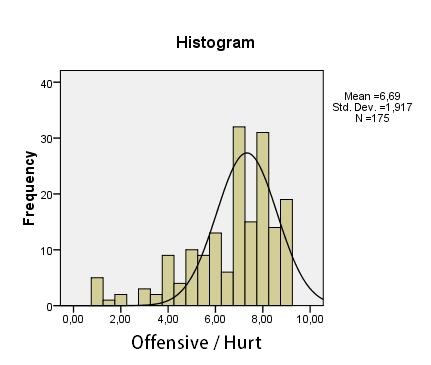
A description of the distribution in the sample suggests that the distribution is very skewed (skewness = -1.14) and that there are clearly more low scores than could be expected from a normal distribution (see histogram below). We should therefore state our reservations about using the t-test here. Given that we do not (yet) have an alternative test, we will interpret the result anyway.
Conclusion: Blogs about the Royal Family are significantly less offensive (M = 4.89, SD = 2.10) than are the other blogs (M = 6.85, SD = 1.82), t (173) = -3.81; p < 0.001; 95% CI [-2.97, -0.94]; d = 1.06. We can conclude with 95% certainty that blogs about the Royal Family score one to three points lower on the offensiveness scale, which runs from 1 (not offensive) to 9 (extremely offensive). This difference is highly relevant, because the effect is considerable. However, we must express a reservation regarding this result: it is not certain whether the distribution of the scores for blogs about the Royal Family have a normal distribution. Below are the manual calculations that have been made to determine the effect size:

and

Syntax
*Recoding the groups.
RECODE Subject (3=1) (ELSE=2) INTO OnderCat.
VARIABLE LABELS OnderCat 'Division of subject: Royal Family versus the rest'.
EXECUTE.
* Define Variable Properties.
*OnderCat.
VALUE LABELS OnderCat
1.00 'Royal Family'
2.00 'Other subjects'.
EXECUTE.
*t-test.
T-TEST GROUPS=OnderCat(1 2)
/MISSING=ANALYSIS
/VARIABLES=Hurt
/CRITERIA=CI(.95).
*Description of the distribution of Hurt in the sample.
*Histogram with normal distribution and skewness.
FREQUENCIES VARIABLES=Hurt
/FORMAT=NOTABLE
/STATISTICS=SKEWNESS SESKEW
/HISTOGRAM NORMAL
/ORDER=ANALYSIS.